 CS 660: Combinatorial Algorithms
Introduction Part B
[To Lecture Notes Index]
San Diego State University -- This page last updated Septemper 3, 1995

- Timing Analysis
- Timing in C on Rohan
- Handling Measurement Errors1
- Estimating Complexity from Timing Results
- Mathematical Analysis and Timing Code
main()
{
- int k, iterations;
- for (iterations = 0; iterations < 50; iterations++)
- {
- start();
- /* start the timer */
- for (k = 0; k < 2000000; k++)
- /* do some work */
- k = k;
- stop();
- /* stop the timer */
-
- printf("Time taken: %ld\n", report());
- };
}
Result on Rohan
Time	Frequency Occurred
30	2
31	2
32	9
33	10
34	11
35	9
36	5
37	1
39	1
Source for Timing C Code on Rohan
#include <stdio.h>
#include <sys/times.h>
#include <limits.h>
static struct tms _start; /* Stores the starting time*/
static struct tms _stop; /* Stores the ending time*/
int start()
{
times(&_start);
}
int stop()
{
times(&_stop);
}
unsigned long report()
{
return _stop.tms_utime - _start.tms_utime;
}
main()
{
int k, iterations;
- for (iterations = 0; iterations < 50; iterations++)
- {
- start();
- /* start the timer */
-
- for (k = 0; k < 2000000; k++)
- /* do some work */
- k = k;
-
- stop();
- /* stop the timer */
-
- printf("Time taken: %ld\n", report());
- };
}
Repeat a measurement n times
Let the measurements be labeled

Let
 and
and

The confidence interval for the true measurement is[2]:

The value of t determine the probability the measurement is in the interval
When n >= 50
Probability	50%	80%	90%	95%	99%
value of t	0.67	1.28	1.64	1.96	2.58
In Example
 ,
s = 3.15, selecting t = 1.96 we get

95% confidence interval is (32.83, 34.57)
Student t table - When n < 50
	n	90%	95%	99%
	1	3.078	6.314	31.821
	2	1.886	2.920	6.965
	3	1.638	2.353	4.541
	4	1.533	2.132	3.747
	5	1.476	2.015	3.365

	6	1.440	1.943	3.143
	7	1.415	1.895	2.998
	8	1.397	1.860	2.896
	9	1.383	1.833	2.821
	10	1.372	1.812	2.764

	20	1.325	1.725	2.528
	30	1.310	1.697	2.457
	40	1.303	1.684	2.423
Fun with Functions
Let f(n) = 3n*n + 4n + 5 and g(n) = 3n*n
Fact: g(n) is an approximation of f(n)
Notation: f(n) = g(n) +

	n	f(n)	g(n)	% error
	1	12	3	75.00%
	10	345	300	13.04%
	20	1285	1200	6.61%
	30	2825	2700	4.42%
	40	4965	4800	3.32%
	50	7705	7500	2.66%
	60	11045	10800	2.22%
	70	14985	14700	1.90%
	80	19525	19200	1.66%
	90	24665	24300	1.48%
	100	30405	30000	1.33%
	200	120805	120000	0.67%
	300	271205	270000	0.44%
Eyeballing Complexity
Let
 then
then
-

Timing Results
	N	Bubble	Insertion
	100	1	1
	200	5	3
	400	19	11
	800	79	42
	1600	317	166
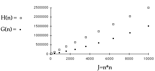
Plotting Complexity
Cubic or Quadratic[3]?
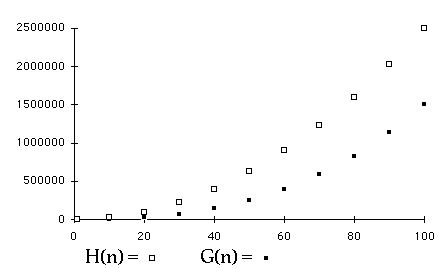 Plotting ComplexityEngineers Method (Modified)
Let
 then
then
-

Let b = 2 and
 then
then
-

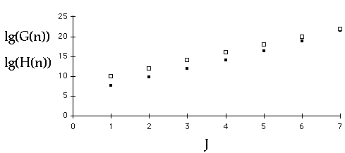 Plotting ComplexityTransform the Axis
Let
 and
and
 (or
(or
 )
then:
g(J) = f(
 )
= a(
 )k
= aJ
So g(J) is linear!
Example
	n	f(n) =5n*n+n + 3	J=n*n
	1	9	1
	10	513	100
	20	2023	400
	30	4533	900
	40	8043	1600
	50	12553	2500
	60	18063	3600

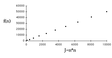 Which is Quadratic?
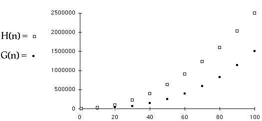
Bubble sort worst case is
 (
n*n )
Complexity is an*n + bn + c
Timing Results Worst Case
	N	Bubble Sort
	400	20
	500	31
	600	45
	700	61
	800	79
Least Squares fit of data to an*n + bn + c
Bubble sort worst case is 0.0001143n*n + 0.01084n - 2.738
Predicted vs. Actual Time for Bubble Sort
	N	Actual	Predicted	% Error
	900	105	99.601	5.14%
	1000	124	122.402	1.29%
	1100	149	147.489	1.01%
	2000	496	476.142	4.00%
	2400	713	681.646	4.40%
 CS 660: Combinatorial Algorithms
 CS 660: Combinatorial Algorithms