 CS660 Combinatorial Algorithms
Fall Semester, 1996
Splay Trees
[To Lecture Notes Index]
San Diego State University -- This page last updated Nov 7, 1996

Contents of Splay Trees
- Self-Organizing BST
- Splay Trees
- Performance of Splay Tree
- Splay Operations
- Top-Down Splay
Basic Rotation
 Simple Exchange (Attempt 1)
When we access a node, apply a rotation to move the node one level closer to
root
If each node is accessed with probability of 1/n the average search time is:

Move-to-root (Attempt 2)
When we access a node, apply series of rotations to make the node the root
We have a list of n items: a1, a2, ..., an
Probability of accessing item ak is P(ak)
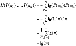
The average search cost is[1]

Where H(P(a1), ....P(an)) is the entropy of the
distribution
If P(ak) = 1/n then
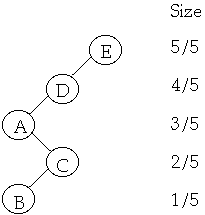
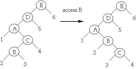
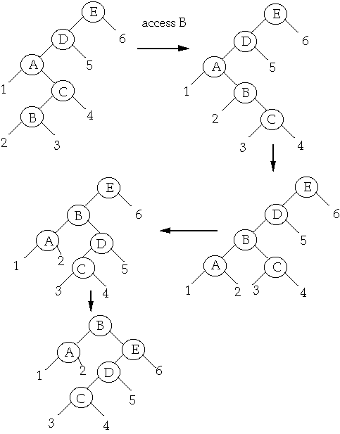
Move-to-root example
Splaying
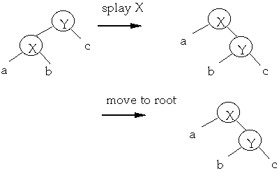
Splay step at x
let p(x) = parent of node x
case 1a (zig) p(x) = root of the tree

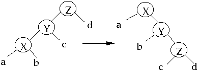
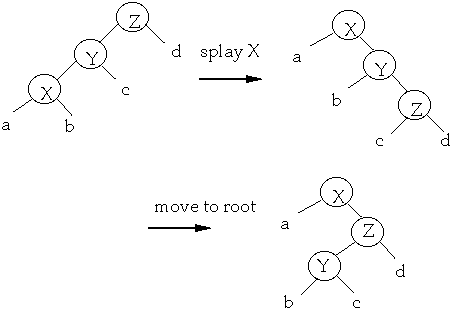
case 2a (zig-zig) p(x) is not the root and x and p(x) are both left
children

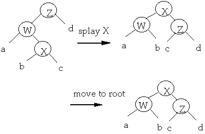
case 3a (zig-zag) p(x) is not the root and x is a left child and p(x)
is a right child
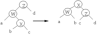
To Splay a node X, repeat the splay step on X until it is the root
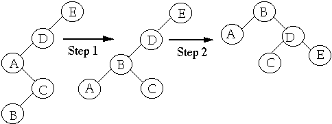
Splay B
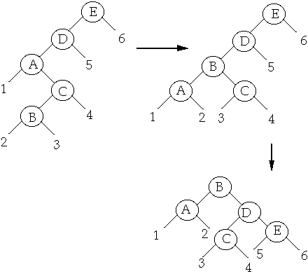
Splay vs. Move-to-root
Case 1
Case 2
Splay vs. Move-to-root
Case 3
Move-to-root A
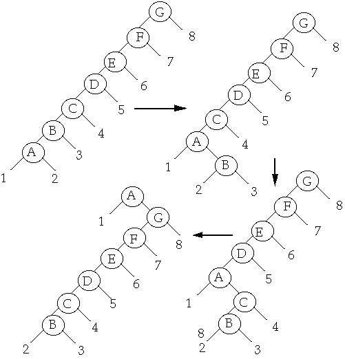
Splay A
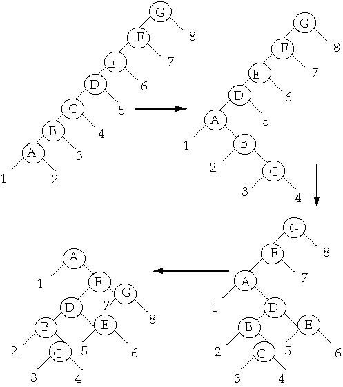
Splaying at a node of depth d takes [[Theta]](d) time
ck= actual cost of operation k
 =
amortized cost of operation k
Dk = the state of the data structure after applying k'th operation
to Dk
 = potential associated with Dk

so we get:
-

-
-
The actual amount of work required is given by:
-
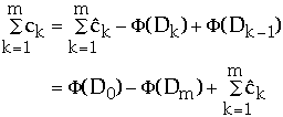
So need the total amortized work and difference in potential
Potential for Splay Trees
Let:
- w(x) = weight of node x, a fixed but arbitrary value
-
 denotes the tree rooted at x
-
 means y is a node in the tree

- size(x) =

- rank(x) = lg(size(x))
-

Example
Let w(x) = 1/n where n is the number of nodes in the tree


Lemma The amortized time to splay node x in a tree with root at t is
at most 3(r(t) - r(x)) + 1 = O(lg(s(t)/s(x)))
- Let s, r denote the size, rank functions before a splay
-
- Let s', r' denote the size, rank functions after a splay
-
- Count rotations
Case 1 (zig) One rotation

Amortized time of this step is:

- = 1 + [r'(x) + r'(y)] - r(x) - r(y)
- only x and y change rank
- <= 1 + r'(x) - r(x)
- r(y) >= r'(y)
- <= 1 + 3(r'(x) - r(x))
- r'(x) >= r(x)
Case 2 (zig-zig) Two rotations

Amortized time of this step is:

- = 2 + r'(x) + r'(y) + r'(z) - r(x) - r(y) - r(z)
-
- only x, y ,z change rank
-
- = 2 + r'(y) + r'(z) - r(x) - r(y)
- r'(x) = r(z)
-
- <= 2 + r'(x) + r'(z) - 2r(x)
- r'(x) >= r'(y) and
-
- r(y) >= r(x)
Assume that 2 <= 2r'(x) - r(x) - r'(z), then
2 + r'(x) + r'(z) - 2r(x) <= 2r'(x) - r(x) - r'(z) + r'(x) + r'(z) -
2r(x)
-
- = 3r'(x) - 3r(x)
-
-
Need to show 2r'(x) - r(x) - r'(z) >= 2
Claim 1

- Set b = 1-a
-
- We have

-
- Setting this to 0 to find extreme value we get
-
-

-
- so
-
-

-
- that is a = 1/2 and b = 1/2
-
- but lg(1/2)+lg(1/2)= -2
End claim 1
Claim 2 2r'(x) - r(x) - r'(z) >= 2
- Recall that:

-
-
- We have:
- r(x) + r'(z) - 2r'(x) = lg(s(x)) + lg(s'(z)) - 2lg(s'(x))
-
-
- = lg(s(x)/s'(x)) + lg(s'(z)/s'(x))
-
- Now s(x) + s'(z) <= s'(x)
- (Why?)
-
- so
- 0<= s(x)/s'(x) + s'(z)/s'(x) <= 1
-
- Set s(x)/s'(x) = a and s'(z)/s'(x) =b in claim 1 to get
-
-
- lg(s(x)/s'(x)) + lg(s'(z)/s'(x)) <= -2
-
Thus r(x) + r'(z) - 2r'(x) <= -2 or 2r'(x) - r(x) - r'(z) >= 2
Case 3 (zig-zag)

Amortized time of this step is:

- = 2 + r'(x) + r'(w) + r'(z) - r(x) - r(w) - r(z)
- <= 2 + r'(w) + r'(z) - 2r(x)
- r'(x) = r(z) and
-
- r(w) >= r(x)
Assume that 2 <= 2r'(x) - r'(w) - r'(z)
2 + r'(w) + r'(z) - 2r(x) <= [2r'(x) - r'(w) - r'(z)] + r'(w) + r'(z) -
2r(x)
= 2r'(x) - 2r(x) <= 3 * ( r'(x) - r(x) )
Claim 3: 2r'(x) - r'(w) - r'(z) >= 2
- Proof: see claims 1 & 2
Putting it All together
Lemma The amortized time to splay node x in a tree with root at t is at
most 3(r(t) - r(x)) + 1 = O(lg(s(t)/s(x)))
Splay at B

Cost of Step 1 <= 3* ( r'(B) - r(B) ) case 3
Cost of Step 2 <= 3 * ( r''(B) - r'(B) ) case 2
Total cost = 3* ( r'(B) - r(B) ) + 3 * ( r''(B) - r'(B) )
- = 3 * ( r''(B) - r(B) )
-
- = 3 * ( r(E) - r(B) )
Case 1 only happens when splaying a child of the root
This happens at most once per splay
Amortized Cost of M Splay Operations
on Tree with N nodes
Let node i be accessed q(i) times.
Then

Theorem (Balance Theorem) The total access time is
- O( (m + n) * lg (n + m) )
Theorem (Static Optimality) If every item is accessed at least once,
then the total access time is:
-

Example
Let q( i ) = 1 then we have

proof of Static Optimality:
Recall that:
- size(x) =

-
- rank(x) = lg(size(x))
-
-

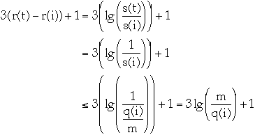
let w(i) = q(i)/m then
-

We wish to compute the actual cost of m operations.
Recall:
-
-

So we need to compute the change in potential and the amortized cost over m
operations.
First the change in potential.
The biggest change in potential comes when a node moves from root to a leaf.
Assume that all nodes start at the root and end up as a leaf.
This will give us an upper bound on the change in potential.
We have:
- rank of the root = lg(W)
-
- rank of node i as a leaf = lg( w( i ) )
So change in rank of node i is at most
- lg(W) - lg( w( i ) ) = lg( W/w(i) )
so the upper bound on the net decrease in potential over m operations is:
-

The amortized access time of item i is:
-

Amortized access of all times is
-

So the total cost is bounded by:
-

access(i, t): if i is in tree t return pointer to i, otherwise return null
pointer
- Find i, then splay tree t at i.
- If i is not in tree t, then splay last node accessed looking for i
join (a, b): Return tree formed by combining tree "a", and tree "b". Assumes
that every item in "a" has key less then every item in "b"
- Splay largest item in "a", then add "b" as a right child of root of "a"
split (i, t): Split tree t, containing item i, into two trees: "a",
containing all items with key less or equal to "i"; and "b", containing all
items with key greater than "i"
- Perform access(i, t) then split tree at root
insert(i, t): insert i in tree t
- Perform split (i, t) then make i the root of the two trees returned by
split
delete(i, t): delete i from tree t
- Perform access(i, t) then perform join on t's subtrees
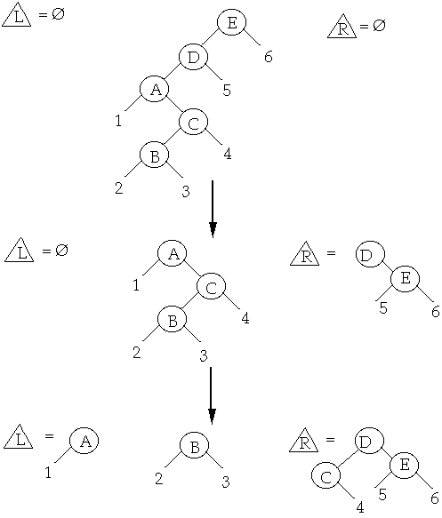
Case 1 X is the node we are splaying

Case 2 (zig-zig) The node we are splaying is in the subtree rooted at
X

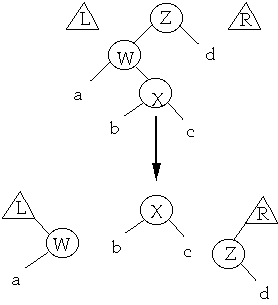
Case 3 (zig-zag) The node we are splaying is in the subtree rooted at
X

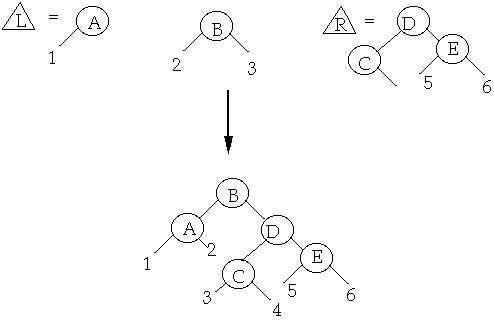
Case 4 - The last step: X is the node we wish to splay

-
Example Splay at B

Example Splay at B

 CS660 Combinatorial Algorithms
 CS660 Combinatorial Algorithms


 =
amortized cost of operation k
 = potential associated with Dk


 denotes the tree rooted at x
 means y is a node in the tree


